Mastering the principles of bagging and boosting with simple examples
Bagging and boosting are two powerful ensemble techniques in machine learning – they are must aware of for data scientists! After analyzing this article, you are going to have a strong understanding of how bagging and boosting work and when to use them. We will cover the following topics, relying heavily on examples to give arms-on illustration of the key principles:
- How Ensembling support create powerful models
- Bagging: Adding stability to ML models
- Boosting: Decreasing bias in weak learners
- Bagging vs. Boosting – while to use each and why
Creating effective models with ensembling
In Machine Learning, ensembling is a wide term that refers to any method that creates predictions by using combining the predictions from a couple of models. If there’s a more than one model involved in creating a prediction, the method is using ensembling!
Ensembling approaches can often improve the overall performance of a single model. Ensembling can assist reduce:
- Variance through averaging multiple models
- Bias by iteratively enhancing on errors
- Overfitting due to the fact the use of a couple of models can growth robustness to spurious relationships
Bagging and boosting are each ensemble strategies which can perform much better than their single-model counterparts. Let’s get into the info of those now!
Bagging: Adding stability to ML models
Bagging is a selected ensembling technique this is used to low the variance of a predictive model. Here, I’m speaking about variance in the machine learning sense – i.e., how much a model varies with changes to the training dataset – no longer variance in the statistical sense which measures the spread of a distribution. Because bagging support lessen an ML model’s variance, it will regularly enhance models that are excessive variance (e.g., decision trees and KNN) however won’t do much excellent for models which can be low variance (e.g., linear regression).
Now that we understand when bagging helps (excessive variance models), allow’s get into the details of the inner workings to recognize how it support! The bagging algorithm is iterative in nature – it builds multiple model by repeating the next three steps:
- Bootstrap a dataset from the original training data
- Train a model at the bootstrapped dataset
- Save the trained model
The collection of models created on this procedure is referred to as an ensemble. When it is time to make a prediction, every model in the ensemble makes its own prediction – the very last bagged prediction is the average (for regression) or majority vote (for classification) of all of the ensemble’s predictions.
Now that we recognize how bagging works, permit’s take a few minutes to build an instinct for why it works. We’ll borrow a acquainted concept from traditional statistics: sampling to estimate a population mean.
In statistics, every sample drawn from a distribution is a random variable. Small sample sizes tend to excessive variance and may provide poor estimates of the true mean. But as we acquire more samples, the average of those samples becomes into a better higher approximation of the population mean.
Similarly, we can assume of each of our individual choice trees as a random variable — in spite of everything, every tree is trained on a different random sample of the data! By averaging predictions from many trees, bagging reduces variance and produces an ensemble model that better captures the true relationships in the data.
Bagging Example
We will be using of the load_diabetes1 dataset from the scikit-learn Python package to illustrate a easy bagging instance. The dataset has 10 input variables – Age, Sex, BMI, Blood Pressure and 6 blood serum degrees (S1-S6). And a single output variable that could be a measurement of disease progression. The code beneath pulls in our data and does a few quite simple cleansing. With our dataset established, let’s start modeling!
# pull in and format data
from sklearn.datasets import load_diabetes

diabetes = load_diabetes(as_frame=True)
df = pd.DataFrame(diabetes.data, columns=diabetes.feature_names)
df.loc[:, 'target'] = diabetes.target
df = df.dropna()
For our example, we are able to use basic choice trees as our base models for bagging. Let’s first confirm that our decision trees are indeed excessive variance. We will do this via training three decision trees on different bootstrapped datasets and observing the variance of the predictions for a check dataset. The graph beneath indicates the predictions of three different decision trees on the identical test dataset. Each three dotted on each line is an individual commentary from the test dataset. The three dots on each line are the predictions from the three different decision trees.
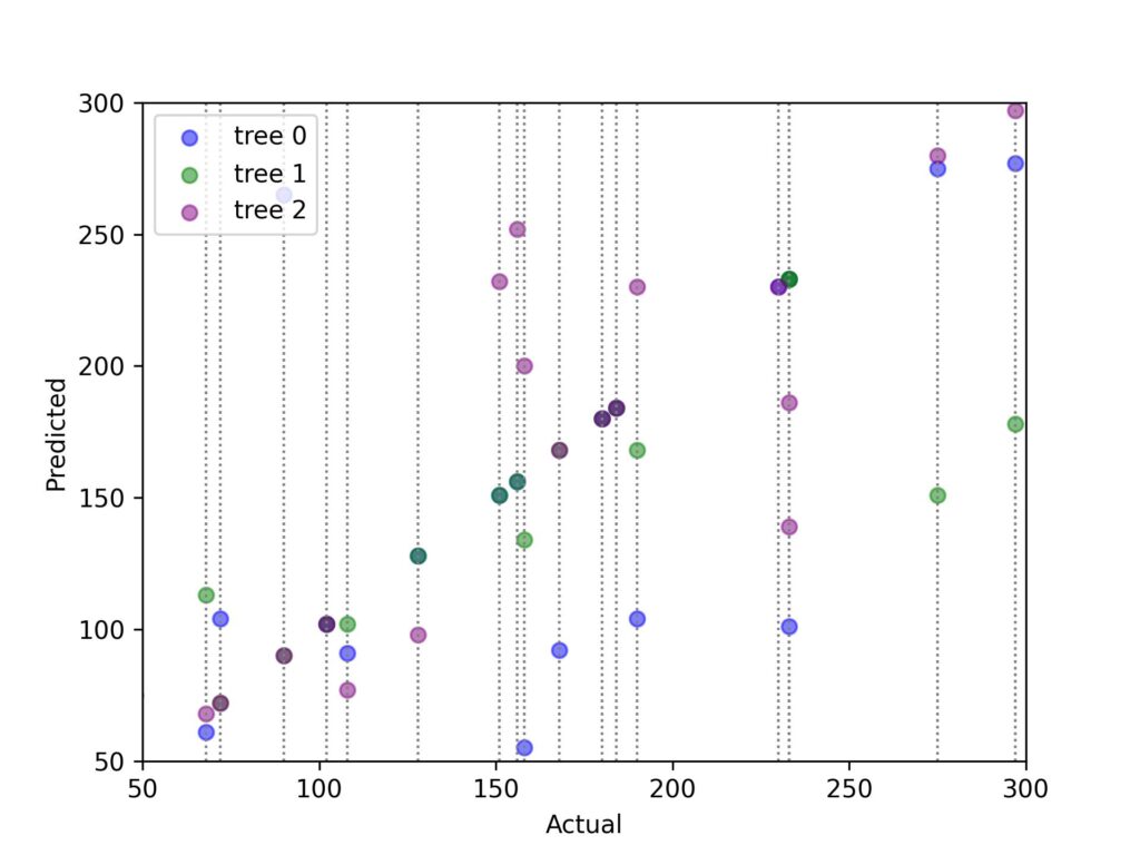
Variance of decision trees on test data points
In the chart above, we see that individuals trees can give very unique predictions (spread of the three dots on every vertical line) whilst trained on bootstrapped datasets. This is the variance we had been talking about!
Now that we see that our trees aren’t very strong to training samples – let’s average the predictions to see how bagging can help! The chart under indicates the average of the three trees. The diagonal line represents best predictions. As you could see, with bagging, our points are tighter and more targeted around the diagonal.
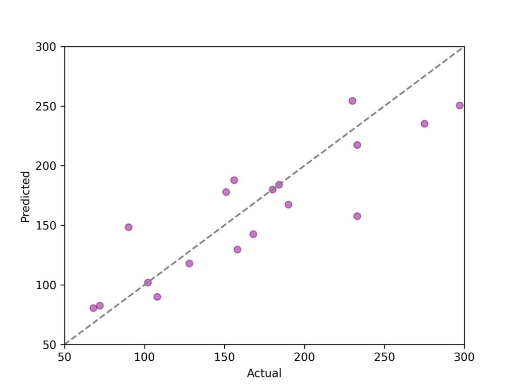
We’ve already seen improvement in our model with the average of simply three trees. Let’s beef up our bagging algorithm with more trees!
Here is the code to bag as many trees as we need:
def train_bagging_trees(df, target_col, pred_cols, n_trees):

    '''
        Creates a decision tree bagging model by training multiple
        decision trees on bootstrapped data.

        inputs
            df (pandas DataFrame) : training data with both target and input columns
            target_col (str)      : name of target column
            pred_cols (list)      : list of predictor column names
            n_trees (int)         : number of trees to be trained in the ensemble

        output:
            train_trees (list)    : list of trained trees

    '''

    train_trees = []

    for i in range(n_trees):

        # bootstrap training data
        temp_boot = bootstrap(train_df)

        #train tree
        temp_tree = plain_vanilla_tree(temp_boot, target_col, pred_cols)

        # save trained tree in list
        train_trees.append(temp_tree)

    return train_trees

def bagging_trees_pred(df, train_trees, target_col, pred_cols):

    '''
        Takes a list of bagged trees and creates predictions by averaging
        the predictions of each individual tree.

        inputs
            df (pandas DataFrame) : training data with both target and input columns
            train_trees (list)    : ensemble model - which is a list of trained decision trees
            target_col (str)      : name of target column
            pred_cols (list)      : list of predictor column names

        output:
            avg_preds (list)      : list of predictions from the ensembled trees

    '''

    x = df[pred_cols]
    y = df[target_col]

    preds = []
    # make predictions on data with each decision tree
    for tree in train_trees:
        temp_pred = tree.predict(x)
        preds.append(temp_pred)

    # get average of the trees' predictions
    sum_preds = [sum(x) for x in zip(*preds)]
    avg_preds = [x / len(train_trees) for x in sum_preds]

    return avg_preds
The functions above are very simple, the first trains the bagging ensemble model, the second takes the ensemble (actually a listing of trained trees) and makes predictions given a dataset.
With our code mounted, let’s run more than one ensemble models and see how our out-of-bag predictions change as we increase the quantity of trees.
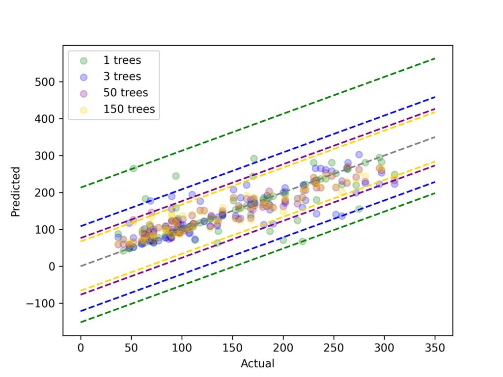
Admittedly, this chart seems a little crazy. Don’t get too bogged down with all of the individual data points, the lines dashed tell the main story! Here we have 1 primary decision tree model and three bagged decision tree models – with 3, 50 and 150 trees. The color-coded dotted lines mark the upper and lower stages for each model’s residuals. There are two main takeaways here:
(1) as we add more trees, the variety of the residuals shrinks and (2) there may be diminishing returns to adding more trees – whilst we go from 1 to 3 trees, we see the range shrink a lot, when we cross from 50 to 150 trees, the range tightens just a little.
Now that we’ve correctly gone via a complete bagging example, we are about ready to move onto boosting! Let’s do a brief evaluation of what we included on this section:
- Bagging reduces variance of ML models with the aid of averaging the predictions of multiple individual models
- Bagging is most beneficial with high-variance models
- The more models we bag, the lower the variance of the ensemble – but there are diminishing returns to the variance reduction benefit
Okay, let’s pass on to boosting!
Boosting: Reducing bias in weak learners
With bagging, we create multiple of independent models – the independence of the models supports average out the noise of individual models. Boosting is likewise an ensembling method; just like bagging, we are able to be training multiple models…. But very different from bagging, the models we train may be dependent. Boosting is a modeling technique that trains an initial model after then sequentially trains additional fashions to improve the predictions of prior models. The primary goal of boosting is to lessen bias – though it may also help lessen variance.
We’ve established that boosting iteratively improves predictions – let’s pass deeper into how. Boosting algorithms can iteratively enhance version predictions in two ways:
- Directly predicting the residuals of the last model and including them to the earlier predictions – think of it as residual corrections
- Adding more weight to the observations that the previous model predicted poorly
Because boosting’s main aim is to reduce bias, it really works properly with base models that commonly have more bias (e.g., shallow choice trees). For our examples, we are going to use shallow decision trees as our base version – we can only cover the residual prediction technique in this article for brevity. Let’s jump into the boosting instance!
Predicting prior residuals
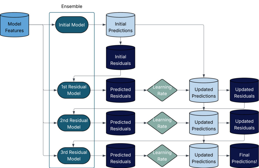
The residuals prediction method begins off with an initial model (a few algorithms offer a steady, others use one iteration of the base model) and we calculate the residuals of that preliminary prediction. The second model in the ensemble predicts the residuals of the first model. With our residual predictions in-hand, we add the residual predictions to our initial prediction (this offers us residual corrected predictions) and recalculate the updated residuals…. We hold this process till we’ve got created the number of base model we specified. This process is quite easy, however is a bit tough to explain with simply words – the flowchart underneath indicates a easy, four-model boosting algorithm.
When boosting, we want to set three main parameters: (1) the number of trees, (2) the tree depth and (3) the learning value. I’ll spend a little time discussing those inputs now.
Number of Trees
For boosting, the range of trees means the same thing as in bagging – i.e., the total number of trees so one can be trained for the ensemble. But, not like boosting, we have to not err on the side of more trees! The chart below shows the test RMSE towards the number of trees for the diabetes dataset.
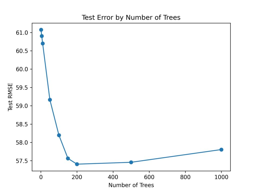
This suggests that the test RMSE drops quickly with the number of trees up till approximately 200 trees, then it starts to creep back up. It seems like a conventional ‘overfitting’ chart – we attain a point wherein more trees turns into worse for the model. This is a key distinction between bagging and boosting – with bagging, more trees eventually stop supporting, with boosting more trees in the end start hurting!
With bagging, more trees eventually stops assisting, with boosting extra trees eventually begins hurting!
We now realize that too many trees are awful, and too few trees are bad as well. We will use hyperparameter tuning to select the variety of trees. Note – hyperparameter tuning is a big subject and way outside of the scope of this article. I’ll exhibit a easy grid search with a train and test dataset for our example a little later.
Tree Depth
This is the maximum depth for each tree in the ensemble. With bagging, trees are frequently allowed to go as deep they want because we’re seeking out low bias, high variance models. With boosting however, we use sequential models to address with the bias in the base learner – so we aren’t as concerned about producing low-bias trees. How can we decide how the most depth? The same technique that we’ll use with the number of trees, hyperparameter tuning.
Learning Rate
The number of trees and the tree depth are acquainted parameters from bagging (even though in bagging we often didn’t put a limit at the tree depth) – however this ‘learning rate’ character is a new face! Let’s take a moment to get familiar. The learning rate is a number between 0 and 1 that is accelerated by way of the current model’s residual predictions before than it is added to the overall predictions.
Here’s a easy example of the prediction calculations with a learning rate of 0.5. Once we understand the mechanics of how the learning rate works, we can discuss the why the learning rate is crucial.
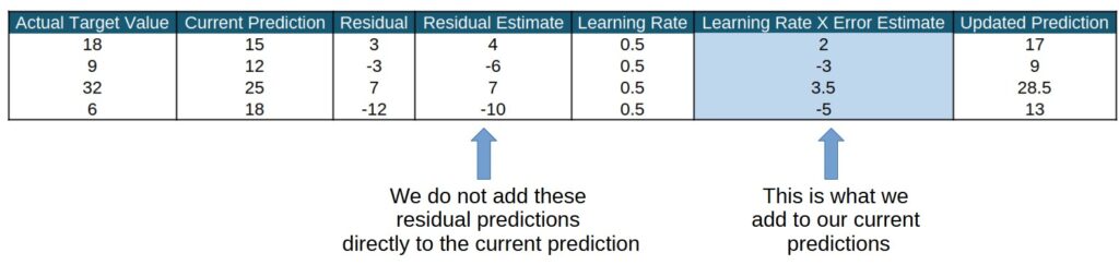
So, why could we need to ‘discount’ our residual predictions, wouldn’t that make our predictions worse? Well, yes and no. For a single generation, it’s going to probably make our predictions worse – however, we are doing a couple of iterations. For more than one iterations, the learning rate keeps the model from overreacting to a single tree’s predictions. It will probable make our modern predictions worse, but don’t worry, we are able to undergo this process a couple of instances! Ultimately, the learning rate supports mitigate overfitting in our boosting model by decreasing the impact of any single tree within the ensemble. You can think of it as slowly turning the steering wheel to correct your driving instead of jerking it. In practice, the number of trees and the learning rate have an opposite relationship, i.e., because the learning rate goes down, the range of trees goes up. This is intuitive, because if we simplest allow a small amount of each tree’s residual prediction to be added to the general prediction, we are going to need a lot more trees before our overall prediction will begin looking good.
Ultimately, the learning rate helps mitigate overfitting in our boosting model by reducing the have an influence of any single tree in the ensemble.
Alright, now that we’ve covered the principle inputs in boosting, let’s get into the Python coding! We need a more than one features to create our boosting algorithm:
- Base decision tree function – a easy function to create and train a single choice tree. We will use the identical function from the last segment called ‘plain_vanilla_tree.’
- Boosting training feature – this function sequentially trains and updates residuals for as many choice trees because the user specifies. In our code, this function is referred to as ‘boost_resid_correction.’
- Boosting prediction function – this characteristic takes a sequence of boosted models and makes final ensemble predictions. We name this function ‘boost_resid_correction_pred.’
Here are the functions written in Python:
# same base tree function as in prior section
def plain_vanilla_tree(df_train,
                       target_col,
                       pred_cols,
                       max_depth = 3,
                       weights=[]):

    X_train = df_train[pred_cols]
    y_train = df_train[target_col]

    tree = DecisionTreeRegressor(max_depth = max_depth, random_state=42)
    if weights:
        tree.fit(X_train, y_train, sample_weights=weights)
    else:
        tree.fit(X_train, y_train)

    return tree

# residual predictions
def boost_resid_correction(df_train,
                           target_col,
                           pred_cols,
                           num_models,
                           learning_rate=1,
                           max_depth=3):
   '''
      Creates boosted decision tree ensemble model.
      Inputs:
        df_train (pd.DataFrame)        : contains training data
        target_col (str)               : name of target column
        pred_col (list)                : target column names
        num_models (int)               : number of models to use in boosting
        learning_rate (float, def = 1) : discount given to residual predictions
                                         takes values between (0, 1]
        max_depth (int, def = 3)       : max depth of each tree model

       Outputs:
         boosting_model (dict) : contains everything needed to use model
                                 to make predictions - includes list of all
                                 trees in the ensemble
   '''


    # create initial predictions
    model1 = plain_vanilla_tree(df_train, target_col, pred_cols, max_depth = max_depth)
    initial_preds = model1.predict(df_train[pred_cols])
    df_train['resids'] = df_train[target_col] - initial_preds

    # create multiple models, each predicting the updated residuals
    models = []
    for i in range(num_models):
        temp_model = plain_vanilla_tree(df_train, 'resids', pred_cols)
        models.append(temp_model)
        temp_pred_resids = temp_model.predict(df_train[pred_cols])
        df_train['resids'] = df_train['resids'] - (learning_rate*temp_pred_resids)

    boosting_model = {'initial_model' : model1,
                      'models' : models,
                      'learning_rate' : learning_rate,
                      'pred_cols' : pred_cols}

    return boosting_model

# This function takes the residual boosted model and scores data
def boost_resid_correction_predict(df,
                                   boosting_models,
                                   chart = False):

   '''
      Creates predictions on a dataset given a boosted model.

      Inputs:
         df (pd.DataFrame)        : data to make predictions
         boosting_models (dict)   : dictionary containing all pertinent
                                    boosted model data
         chart (bool, def = False) : indicates if performance chart should
                                     be created
      Outputs:
         pred (np.array) : predictions from boosted model
         rmse (float)    : RMSE of predictions
   '''

    # get initial predictions
    initial_model = boosting_models['initial_model']
    pred_cols = boosting_models['pred_cols']
    pred = initial_model.predict(df[pred_cols])

    # calculate residual predictions from each model and add
    models = boosting_models['models']
    learning_rate = boosting_models['learning_rate']
    for model in models:
        temp_resid_preds = model.predict(df[pred_cols])
        pred += learning_rate*temp_resid_preds

    if chart:
        plt.scatter(df['target'],
                    pred)
        plt.show()

    rmse = np.sqrt(mean_squared_error(df['target'], pred))

    return pred, rmse
Sweet, lets make a model on the identical diabetes dataset that we used within the bagging section. We’ll do a quick grid search (again, no doing some thing fancy with the tuning here) to tune our three parameters after which we’ll train the very last model using the boost_resid_correction feature.
# tune parameters with grid search
n_trees = [5,10,30,50,100,125,150,200,250,300]
learning_rates = [0.001, 0.01, 0.1, 0.25, 0.50, 0.75, 0.95, 1]
max_depths = my_list = list(range(1, 16))

# Create a dictionary to hold test RMSE for each 'square' in grid
perf_dict = {}
for tree in n_trees:
    for learning_rate in learning_rates:
        for max_depth in max_depths:
            temp_boosted_model = boost_resid_correction(train_df,
                                                        'target',
                                                         pred_cols,
                                                         tree,
                                                         learning_rate=learning_rate,
                                                         max_depth=max_depth)
            temp_boosted_model['target_col'] = 'target'
            preds, rmse = boost_resid_correction_predict(test_df, temp_boosted_model)
            dict_key = '_'.join(str(x) for x in [tree, learning_rate, max_depth])
            perf_dict[dict_key] = rmse

min_key = min(perf_dict, key=perf_dict.get)
print(perf_dict[min_key])
And our winner is 🥁— 50 trees, a learning rate of 0.1 and a max depth of 1! Let’s take a look and see how our predictions did.
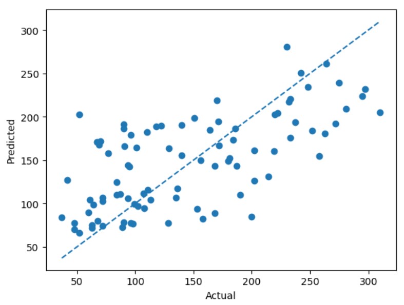
While our boosting ensemble model seems to capture the trend reasonably well, we can see off the bat that it isn’t predicting as well as the bagging model. We could probably spend more time tuning – but it could also be the case that the bagging approach fits this specific data better. With that said, we’ve now earned an understanding of bagging and boosting – let’s compare them in the next section!
Bagging vs. Boosting – understanding the differences
We’ve covered bagging and boosting separately, the table below brings all the information we’ve covered to concisely compare the approaches:
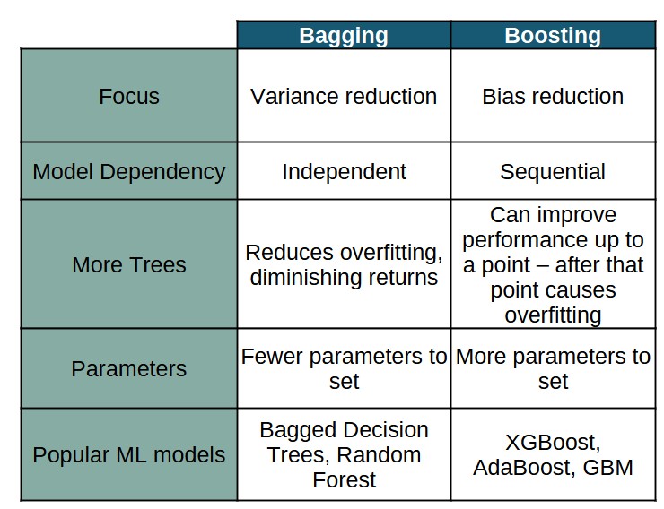
Note: In this article, we wrote our own bagging and boosting code for educational purposes. In practice you will just use the excellent code that is available in Python packages or other software. Also, people rarely use ‘pure’ bagging or boosting – it is much more common to use more advanced algorithms that modify the plain vanilla bagging and boosting to improve performance.
Wrapping it up
Bagging and boosting are powerful and practical ways to improve weak learners like the humble but flexible decision tree. Both approaches use the power of ensembling to address different problems – bagging for variance, boosting for bias. In practice, pre-packaged code is almost always used to train more advanced machine learning models that use the main ideas of bagging and boosting but, expand on them with multiple improvements.
I hope that this has been helpful and interesting – happy modeling!